Transformer Is Inherently a Causal Learner

Xinyue Wang · Halıcıoğlu Data Science Institute, University of California San Diego

Stephen Wang · ABEL Intelligence, Inc. · Mountain View, CA 94040

Biwei Huang · Halıcıoğlu Data Science Institute, University of California San Diego

Abstract

We reveal that transformers trained in an autoregressive manner naturally encode time-delayed causal structures in their learned representations. When predicting future values in multivariate time series, the gradient sensitivities of transformer outputs with respect to past inputs directly recover the underlying causal graph, without any explicit causal objectives or structural constraints. We prove this connection theoretically under standard identifiability conditions and develop a practical extraction method using aggregated gradient attributions. On challenging cases such as nonlinear dynamics, long-term dependencies, and non-stationary systems, this approach greatly surpasses the performance of state-of-the-art discovery algorithms, especially as data heterogeneity increases, exhibiting scaling potential where causal accuracy improves with data volume and heterogeneity, a property traditional methods lack. This unifying view lays the groundwork for a future paradigm where causal discovery operates through the lens of foundation models, and foundation models gain interpretability and enhancement through the lens of causality.

Introduction

The ability to discover causality is foundational to intelligence, enabling understanding, prediction, and decision-making about the world. As an evolving field, causal discovery aims to formalize theoretical frameworks for identification criteria and to propose search algorithms to find the true causal structure from observational data. In this area, causal discovery from time series focuses on identifying temporal causal dynamics by exploiting the temporal ordering that naturally constrains the direction of causation. Granger causality formalizes this intuition: a variable $X$ Granger-causes $Y$ if past values of $X$ contain information that helps predict $Y$ beyond what is available from past values of $Y$ alone. Additional methods extend this foundation, including constraint-based approaches like PCMCI and its variants that iteratively test conditional independence to examine the existence of causal edges, score-based methods like DYNOTEARS that optimize graph likelihood with structural prior regularizations, and functional approaches like TiMINo and VAR-LiNGAM that leverage structural equation models and non-Gaussianity for identifiability.

Real-world systems exhibit complex interactions among many variables. For example, financial markets are highly non-stationary and involve very large variable sets; neural recordings exhibit strongly nonlinear population dynamics; climate sensor networks display long and short-term teleconnections; and unstructured modalities such as video require modeling long-range spatiotemporal dependencies. Despite rigorous theoretical foundations, prevailing algorithms are often constrained in practice by complex heuristics. Specifically, constraint-based and score-based approaches scale poorly: the number of statistical tests grows rapidly with dimension and lag, and non-parametric tests are computationally expensive. Optimization approaches require careful tuning to achieve the right balance between likelihood and structural regularization. More fundamentally, these estimators are not scalable representation learners: their learning is not transferable and thus offers little generalizability for zero-shot or few-shot adaptation; their effective capacity and expressiveness are not well-suited for pretraining on diverse systems.

Motivated by the striking performance and scaling behavior of autoregressive foundation models, we ask whether the properties that make transformers strong forecasters can help causal discovery. Building this connection is valuable in two directions: for discovery, it promises data efficiency by leveraging pretrained representations and a scalable learning paradigm suited to complex dependencies; for foundation models, causal principles offer ways to diagnose limitations in memory and hallucinations, and guide architecture and objective choices. In this paper, we take a first step toward these goals: we revisit common identifiability assumptions in lagged data generation processes and show how decoder-only transformers trained for forecasting, together with input–output gradient attributions via Layer-wise Relevance Propagation (LRP), reveal lagged causal structure. This view turns modern sequence models into practical, scalable estimators for temporal graphs while opening a path to analyze and strengthen foundation models through causal perspectives.

Background

Related Work

Time-series Causal Discovery. Recovering causal dynamics from temporal observations requires structural assumptions that determine when and how the true causal graph is identifiable. Constraint-based methods, assuming causal sufficiency and faithfulness, prune spurious edges via conditional independence tests. PCMCI and its variants extend the PC algorithm to handle nonlinear, contemporaneous, non-stationary, and high-dimensional settings. Score-based methods search for structures that optimize scores encoding functional form and complexity preferences, with recent continuous relaxations reducing computational cost. Functional methods exploit noise asymmetry to resolve edge orientation: VAR-LiNGAM assumes linear dynamics with non-Gaussian noise, while TiMINo generalizes to nonlinear additive-noise processes. Granger causality tests whether past values of one series improve forecasts of another, reflecting predictive rather than structural causation; neural extensions handle nonlinear dependencies.

Transformer Interpretability. The success of large-scale pretrained transformers has motivated diverse interpretability efforts. Most relevant to our work are methods for input–output token attribution in autoregressive models. Early work equated attention with explanation, but attention proves manipulable and misaligned with perturbation effects. Post-processing techniques like attention rollout aggregate across layers and heads, yet remain forward-weight heuristics rather than faithful causal measures. Gradient-based methods such as saliency, Integrated Gradients, and Layer-wise Relevance Propagation estimate output-conditioned sensitivities through attention, residual, and MLP paths, yielding attributions that better align with perturbation tests. We ground token-level attributions in identifiability theory for dynamic systems, providing a causally principled framework for interpreting transformers as structure learners.

Motivations

Modern scientific and industrial systems are high-dimensional, nonlinear, non-stationary, and data-rich — precisely the regime where classical causal discovery faces brittle assumptions, exploding conditioning sets, and poor scaling with many variables, long lags, and complex dependencies. Decoder-only transformers sit at the opposite point in the design space: a single autoregressive objective, contextualized dependency modeling, and predictable gains from scale, data, and compute. Empirically, the same architecture transfers across modalities and domains and often outperforms specialized models in text, vision, and long-context time series. Our premise is pragmatic: if many real-world regularities arise from a small set of sparse, independent mechanisms, then an autoregressive learner that already scales and generalizes is a natural interface to structure learning.

This brings three immediate benefits: (i) amortization — forecasting supplies a ubiquitous training signal, turning structure learning into a unified, scalable procedure grounded in identifiability insights; (ii) the long-term potential of leveraging pretrained priors to reduce sample complexity when moving to new domains; and (iii) coverage — complex nonlinear, long-term dependencies and a diverse set of dynamic systems are handled within a unified framework.

A Unifying View: Identification inside Robust Next Variables Prediction

From Prediction to Causation

Data-generating process. Consider a $p$-variate time series $X_t = (X_{1,t}, \ldots, X_{p,t})^\top$ and a lag window $L \ge 1$. Each variable follows

$X_{i,t} = f_i(\text{Pa}(i,t), U_{t}, N_{i,t}),$

where $\text{Pa}(i,t) \subseteq \{X_{j,t-\ell} : j \in [p],\, \ell \in [L]\}$ are the lagged parents, $U_{t}$ are unobserved processes, and $N_{i,t}$ are mutually independent noises satisfying $N_{i,t} \perp (X_{1:t-1}, U_{\leq t})$. We write $j \stackrel{\ell}{\longrightarrow} i$ if $X_{j,t-\ell}$ is a direct cause of $X_{i,t}$. The lagged graph $\mathcal{G}^*$ contains $j \stackrel{\ell}{\longrightarrow} i$ if and only if $X_{j,t-\ell} \in \text{Pa}(i,t)$.

Assumptions for lagged identifiability:

• A1 Conditional Exogeneity.
• A2 No instantaneous effects (all parents occur at lags $\ell \ge 1$).
• A3 Lag-window coverage (the chosen $L$ includes all true parents).
• A4 Faithfulness (the distribution is faithful to $\mathcal{G}^*$).

Causal Identifiability via Prediction. Under A1–A4 and regularity conditions, the lagged causal graph $\mathcal{G}^*$ is uniquely identifiable via the score gradient energy. In particular, the edge $j\,\stackrel{\ell}{\longrightarrow}\, i$ exists if and only if

$H_{j,i}^{\ell} := \mathbb{E}\left[ \left( \partial_{x_{j,t-\ell}} \log p\left(X_{i,t} \mid X_{1:t-1}\right) \right)^2 \right] > 0.$

This theorem characterizes causal parents through sensitivity of the conditional distribution to each input. Unlike classical Granger causality, which tests mean prediction, the score gradient energy $H_{j,i}^{\ell}$ captures influence on the entire conditional distribution, including variance and higher moments. Under homoscedastic Gaussian noise, this reduces to $G_{j,i}^{\ell} := \mathbb{E}[({\partial_{x_{j,t-\ell}} f^*(X_{i,t})})^2]$, where $G_{j,i}^{\ell} > 0$ iff edge $j \stackrel{\ell}{\to} i$ exists.

Transformers Inherit Causal Identifiability

We connect the theorem to decoder-only transformers and make explicit why this architecture aligns with the identifiability program, and how we extract a graph in practice. The connection has four parts.

Alignment with identifiability and objective. We use a decoder-only transformer on a length-$L$ window. For each $t>L$, the input $\mathbf{s}_t=[X_{t-L},\ldots,X_{t-1}]\in\mathbb{R}^{L\times p}$ is flattened to $L\cdot p$ tokens. We use separate learnable node and time embeddings to distinguish temporal positions and node identities. Causal masking and autoregressive decoding enforce temporal precedence (A2); the window $L$ bounds the maximum lag (A3). We optimize:

$\min_{\theta}\; -\frac{1}{(T-L)\,L}\sum_{i=1}^{T-L}\sum_{k=1}^{L} \log p_{\theta}\!\left(X_{i+k}\,\middle|\,X_{i:i+k-1}\right) \;+\; \lambda\,\Omega(\theta).$

where $p_{\theta}(\cdot\mid\cdot)$ denotes the conditional likelihood parameterized by transformer outputs $\widehat{f}_\theta: \mathbb{R}^{L\times p} \to \mathbb{R}^p$.

Sparsity and scalable dependence selection. While explicit sparsity is not required for identifiability in the population, finite-sample recovery benefits from sparsity for both accuracy and efficiency. Transformers implicitly sparsify: finite capacity, weight decay compress high-dimensional observations into generalizable parameters; softmax attention induces competitive selection among candidates; and multi-head context supports selecting complementary parents.

Attention as contextual parameters. Attention matrices are input-conditioned and therefore act as contextualized parameters of pairwise dependencies rather than fixed population-level graph weights. Unlike methods that learn a single static binary mask, input-conditioned attention adapts to heterogeneity and non-stationarity: different contexts (time, regime) induce distinct effective dependency patterns.

Structure extraction. After training, we recover the structure via population gradient energy rather than raw attention. We use LRP to compute relevance scores $R_{ij}^{(\ell)}$ that quantify the influence of variable $j$ at lag $\ell$ on predicting variable $i$ at time $t$:

$R_{ij}^{(\ell)} \,=\, \sum_{m=1}^M \sum_{h=1}^H \mathrm{LRP}^{(m,h)}\big(\widehat{f}_\theta, X_t^{(i)}, X_{t-\ell}^{(j)}\big).$

We aggregate these attributions across samples to estimate gradient energy $\tilde G_{j,i}^{(\ell)}=\mathbb{E}[\,|R_{ij}^{(\ell)}(X)|\,]$ and then calibrate to a sparse graph.

Graph binarization. We propose two rules to binarize $\tilde G$: (i) Top-$k$ per target: for each target variable (row), select the $k$ largest entries as parents; this directly controls graph density and stabilizes precision. (ii) Uniform-threshold rule: assume a uniform baseline over $L \times p$ candidates and select entries whose normalized relevance exceeds $\tfrac{1}{L \times p}$.

Why gradients rather than raw attention. Tokens in deep transformer layers are highly contextualized and are heavily mixed by downstream value projections and residual paths. Consequently, large attention on a token does not guarantee a large effect on the target, and deep mixing can obscure true dependencies. In contrast, gradients directly quantify local sensitivity of the target to each input coordinate; integrating their magnitude over the data yields a population-level measure aligned with our identifiability results.

Experiments

Simulation Experiments

Figure 1: Data generation and transformer-based causal discovery.

Setup. We evaluate our procedure for causal discovery using simulated datasets. We construct datasets along several axes, including high-dimensional inputs, long-range dependencies, nonlinear interactions, non-stationary processes, unobserved latent variables, and different exogenous noise types. We compare against baselines from a diverse set of algorithm families including PCMCI, DYNOTEARS, VAR-LiNGAM, NTS-NOTEARS, TCDF, pairwise/multivariate Granger tests, and a random guess baseline based on the ground-truth density. After training, we extract edges with LRP and binarize them with a per-target top-$k$ rule to obtain an inferred causal structure, and then evaluate performance using the F1 score.

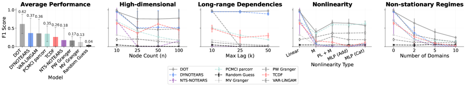Figure 2: F1 score analysis across regimes.

General capabilities. The transformer recovers lagged parents accurately and consistently across settings, achieving comparable or better performance to baseline methods. The transformer maintains consistent and strong performance in all settings, where specialized approaches perform well in some settings but worse in others. Traditional methods degrade as dynamics and dimension grow, whereas the transformer remains robust without sensitive hyperparameter tuning.

Figure 3: Nonlinear dependencies sample scaling.

Capabilities of modeling long-range and high-dimensional dependencies. The attention mechanism connects any pair of variables in one hop, making it excel at modeling long-range and complicated connections of a high-dimensional system. Decoder-only transformers consistently surpass baselines in both high-dimensional and long-range dependency settings. Traditional algorithms like VAR-LiNGAM and PCMCI perform worse when the input dimension increases, suffering from weaker detection power and the curse of dimensionality.

Capabilities of modeling nonlinear interactions. We observe a trade-off between data efficiency and expressivity. While traditional methods employing simple estimators and search heuristics from human prior (e.g., DYNOTEARS, VAR-LiNGAM, PCMCI) can achieve good performance efficiently in simple cases like linear settings, a decoder-only transformer generally works better when the data scales and shows a consistent accuracy improvement as data increases.

Figure 4: Non-stationary dependencies sample scaling.

Scaling behavior in non-stationary settings. The transformer can effectively leverage additional data to improve causal structure estimation accuracy. Unlike traditional methods that can become intractable as data grows, the transformer shows consistent improvement across sample sizes. In non-stationary settings, the model learns to handle multiple local mechanisms within a single framework.

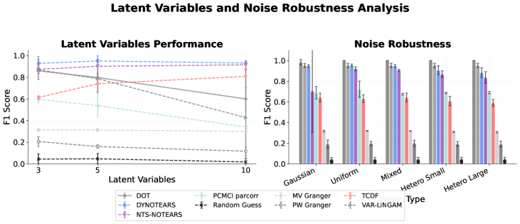Figure 5: Robustness to latent variables and noise.

Noise and latent variable robustness. Transformers demonstrate robust performance across different noise distributions, maintaining consistent accuracy regardless of noise type or the variance properties of noise. However, due to the lack of a latent variable modeling mechanism, transformers are prone to learn spurious links and degrade as the number of latent variables increases.

Figure 6: Post-processing for latent confounders, instantaneous relationships, and domain indicators.

The potential of handling latent confounders. Transformer performance degrades under latent confounding, and the architecture cannot generally model latent variables. We show that it is possible to handle this by post-processing with a latent-aware causal discovery method: run L-PCMCI constrained by the transformer's predicted edges to refine the graph. Starting from the transformer's graph sharply reduces the expensive search space of latent-aware causal discovery methods.

The potential of handling instantaneous relationships. The decoder-only transformer lacks the ability to model instantaneous relationships due to its autoregressive nature. We combine the transformer's learned lagged structure with a fully connected contemporaneous graph and use it as the initial skeleton for PCMCI+, which refines the confounded lagged graph and identifies instantaneous relationships.

Figure 7-9: Uncertainty analysis examples in the linear setting.

Attention and gradient attribution. We find that the relationship between attention scores and gradient-based attributions differs for deep and shallow transformers. In deep transformers, attention scores reveal little information about the learned structure, while in one-layer transformers, structures extracted from attention are much more accurate and better aligned with LRP outputs.

Figure 10: Transformer variants performance comparison on challenging regimes.

The effect of model depth. With more layers, the transformer can model more complex structures and longer-range effects. Deeper transformers achieve higher accuracy in recovering causal structure and show clear advantages with LRP readout.

Figure 11: Intervention effects and gradient-based attributions in the linear case.

Real-World Experiments

We compare the decoder-only transformer (DOT) with a series of time-series causal discovery methods on the CausalTime dataset. The CausalTime benchmark includes three datasets and corresponding prior graphs for real-world air quality, traffic, and medical scenarios.

Method	AQI AUROC	AQI AUPRC	Traffic AUROC	Traffic AUPRC	Medical AUROC	Medical AUPRC
GC	0.454	0.635	0.419	0.279	0.574	0.421
SVAR	0.623	0.790	0.633	0.585	0.713	0.677
PCMCI	0.527	0.673	0.542	0.347	0.699	0.508
CUTS+	0.893	0.798	0.618	0.637	0.820	0.548
LCCM	0.857	0.926	0.555	0.591	0.801	0.755
JRNGC-F	0.928	0.783	0.729	0.594	0.754	0.726
DOT (Ours)	0.866	0.699	0.703	0.570	0.724	0.651
MLP (Ours)	0.913	0.752	0.635	0.481	0.872	0.826

Although DOT is optimized for prediction rather than structure learning, it surpasses most traditional causal discovery methods and ranks among the top three on the air-quality and traffic datasets. This suggests the potential of a prediction-first strategy for causal discovery in the real world.

Appendix

Identifiability of the Causal Structure

We formalize when gradients of the conditional distribution recover the lagged causal parents. For a fixed target $Y := X_{i,t}$, we write $H_j$ for the score gradient energy. Consider the structural equation:

$X_{i,t} = f_i(\text{Pa}(i,t), U_{t}, N_{i,t}), \quad i = 1, \ldots, p,$

Define the score of the conditional density:

$s(y,x) := \nabla_x \ell^*(y,x), \qquad s_j(y,x) := \partial_{x_j} \ell^*(y,x),$

and the score gradient energy:

$H_j := \mathbb{E}\Big[(s_j(Y,X))^2\Big], \quad j=1,\ldots,d.$

Theorem (Score-based characterization of lagged parents). Under the data generating process, conditional exogeneity, no instantaneous effects, Causal Markov and Faithfulness, and conditional density regularity assumptions, the score gradient energy $H_j$ recovers the full lagged structural parent set:

$H_j=0 \;\iff\; j\notin S.$

In particular, if $k\in S$ then $H_k>0$.

Special Case: Homoscedastic Additive Gaussian Noise

Under homoscedastic additive Gaussian noise with $Y_t = f(X_S) + \epsilon$ and $\epsilon \sim \mathcal{N}(0,\sigma_0^2)$, the score gradient energy satisfies:

$H_j = \frac{G_j}{\sigma_0^2}.$

where $G_j := \mathbb{E}\left[({\partial_{x_j} f(X_S)})^2\right]$. Since $\sigma_0>0$, we have $H_j=0$ if and only if $G_j=0$.

Corollary. Under the homoscedastic additive Gaussian noise model together with all assumptions from the main theorem, the gradient energy $G_j$ recovers the full lagged structural parent set: $G_j=0 \;\iff\; j\notin S.$

Attention LRP as a Surrogate for Gradient Energy

For a trained forecaster $\hat f$ and a scalar prediction $z:=\hat f(x)$, per-sample relevance is defined as:

$R(x) := x \;\odot\; \widetilde{\nabla}_{x} z,$

where $\widetilde{\nabla}_{x}$ denotes a gradient computed with modified local Jacobians. Aggregating coordinates gives a global score:

$\tilde G_j := \mathbb{E}\big[\,|R_j(X)|\,\big],$

used as a monotone proxy for $G_j=\mathbb{E}[(\partial_{x_j} f^*(X))^2]$.

Training Details and Model Architecture

We train autoregressive transformers on lag-$K$ windows after per-variable z-score normalization. We use an embedding dimension of 64, 4 attention heads, and either 1 ("shallow") or 4 ("deep") layers with pre-LayerNorm, residual connections, and a 2-layer ReLU feed-forward network, together with causal masking and node/time embeddings. Models are optimized with Adam (learning rate $10^{-3}$, batch size 256) under an MSE objective.

Additional Figures

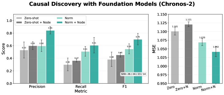Figure 12: Structure recovery with Chronos2 on linear data.

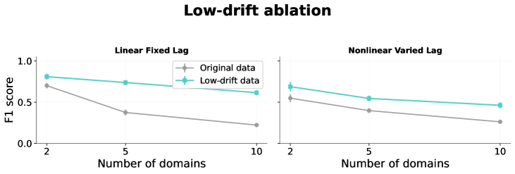Figure 13: Performance under non-stationary settings with minimal changes across regimes.

Figure 14: Sensitivity to k in row-wise top-k binarization.

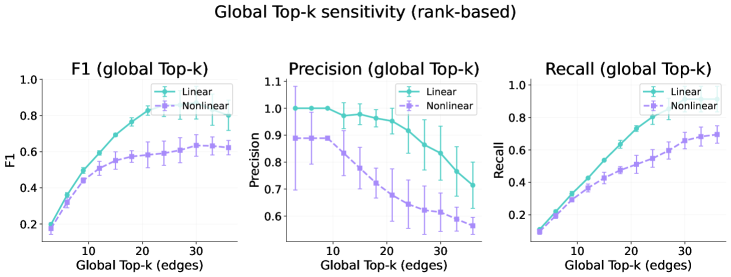Figure 15: Sensitivity to k in global top-k binarization.

Figure 16: Convolutional neural network as an alternative to transformer predictor.

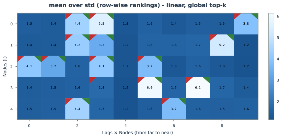
Figure 17-25: Extended uncertainty analysis in linear settings.

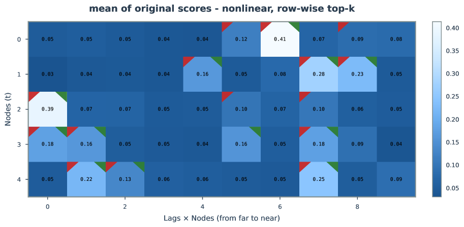
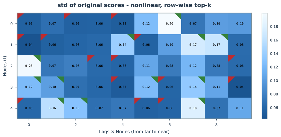
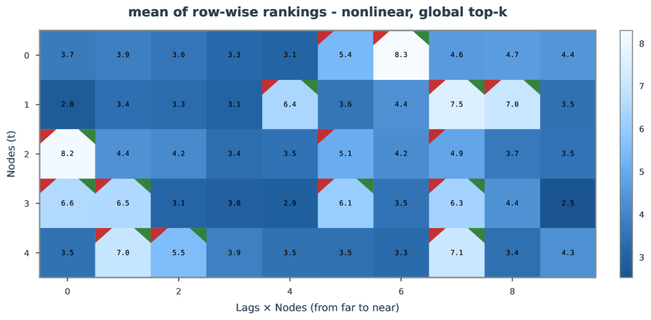
Figure 26-33: Extended uncertainty analysis in nonlinear settings.

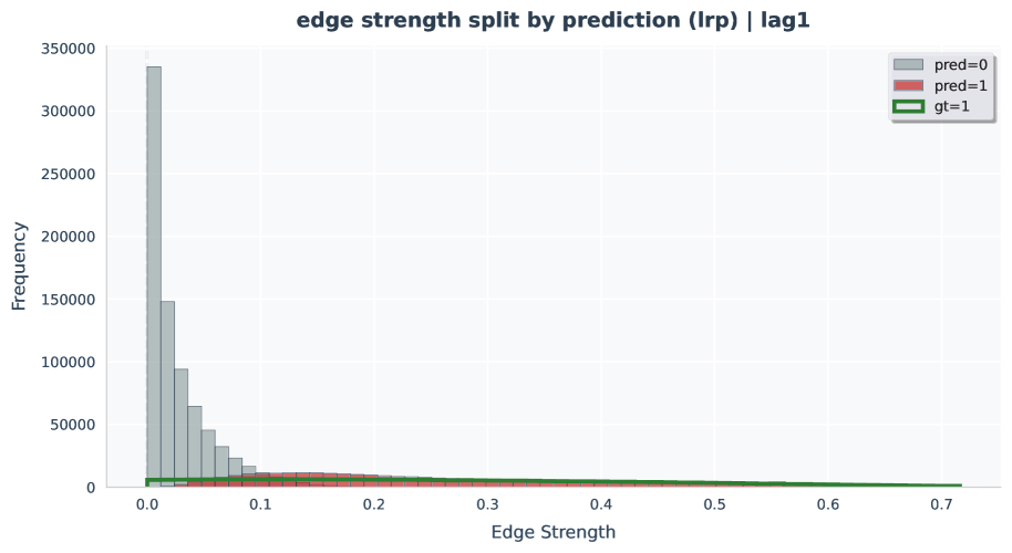
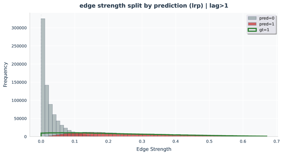
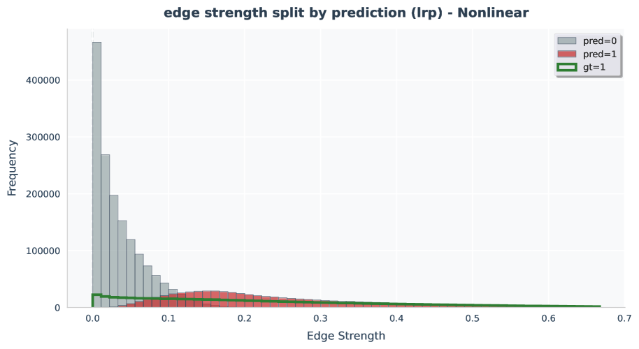
Figure 34-39: Edge-strength histogram analyses.

Conclusion

We ask whether modern sequence models can reveal causal structure while learning to forecast. We prove that, under standard assumptions, decoder-only transformers trained autoregressively admit causal identifiability: the output's sensitivities to lagged inputs recover the true parents. We operationalize this with an aggregated gradient-energy readout (LRP) and a simple top-$k$ binarization. Across nonlinear, long-range, high-dimensional, and non-stationary regimes, this procedure surpasses strong baselines and improves monotonically with data. This reframes discovery as a by-product of scalable representation learning while giving foundation models a causal lens. In sum, transformers are not only strong forecasters: read out with gradients, they are scalable causal learners, and causality, in turn, offers principled guidance to make foundation models more robust, data-efficient, and interpretable.